
Disk is the data plane: Flight Shuffle in Daft
How Daft rebuilt distributed shuffle around Arrow Flight, local disk, and streaming reads to handle multi-terabyte workloads.
by Colin Ho, Chris KelloggIf you scale a distributed query to tens of terabytes, one operation will dominate everything else:
The shuffle.
Daft's original distributed shuffle used Ray's in-memory object store as its transport layer. It worked well for moderate workloads, but broke down on large-scale jobs that created 10+ TB shuffles with thousands of output partitions.
The bottleneck wasn't bandwidth, but the coordination and memory overhead of modeling a shuffle as millions of distributed in-memory objects. So we rebuilt the shuffle stack from scratch.
Flight Shuffle is Daft's new disk-backed, streaming shuffle algorithm.
Map tasks write Arrow IPC straight to local disk, while reduce tasks fetch partitions over Arrow Flight RPC and stream them into the executor without ever materializing a whole partition in memory.
The shuffle, and why it is hard
Up to the shuffle, every worker processes its own slice of data and never has to talk to the others. The shuffle is where that stops. In a group-by aggregation, for example, rows with the same group-by key need to be located on the same worker, therefore requiring a shuffle to redistribute data.
Anything that reorganizes data globally becomes a shuffle:
# Repartition
df = df.repartition(4096, "episode_id")

# Hash join
joined = events.join(metadata, on="trajectory_id")

# Grouped aggregation
agg = df.groupby("scene_id").agg(col("force").mean())

# Global sort
df = df.sort("timestamp")
A shuffle stresses every subsystem at once. CPUs hash and partition records, memory buffers in-flight data, disks spill what doesn't fit, the network moves partitions between workers, and the scheduler tracks the transfers. The hard part is keeping all of those balanced. If disk writes fall behind, memory pressure builds. If the scheduler drowns in partition metadata, the pipeline stalls before the network is ever saturated.
And the cost scales with partition count. An M-mapper, N-reducer shuffle creates M x N logical connections: every reducer pulls from every mapper. At 4096 x 4096, that's over 16 million transfers.
That's exactly the shape of the workloads we kept hitting: repartitioning multimodal datasets by episode, joining fleet telemetry against trajectory metadata, aggregating embeddings and sensor streams across hundreds of billions of rows. At that scale, the shuffle architecture itself becomes the limiting factor.
The old approach: Ray's in-memory object store as the shuffle data plane
Daft's distributed engine uses Ray to orchestrate tasks and workers, and it also used Ray's in-memory object store (a shared memory pool across the cluster) to transfer data between workers.
Map tasks partitioned their output by key and wrote each partition into the Ray object store. Reduce tasks retrieved their respective partitions with ray.get, reconstructed them in memory, and handed them to the executor. Every shuffle partition became a distributed object that the control plane had to track, and that coordination runs centrally on the cluster's head node (the driver).
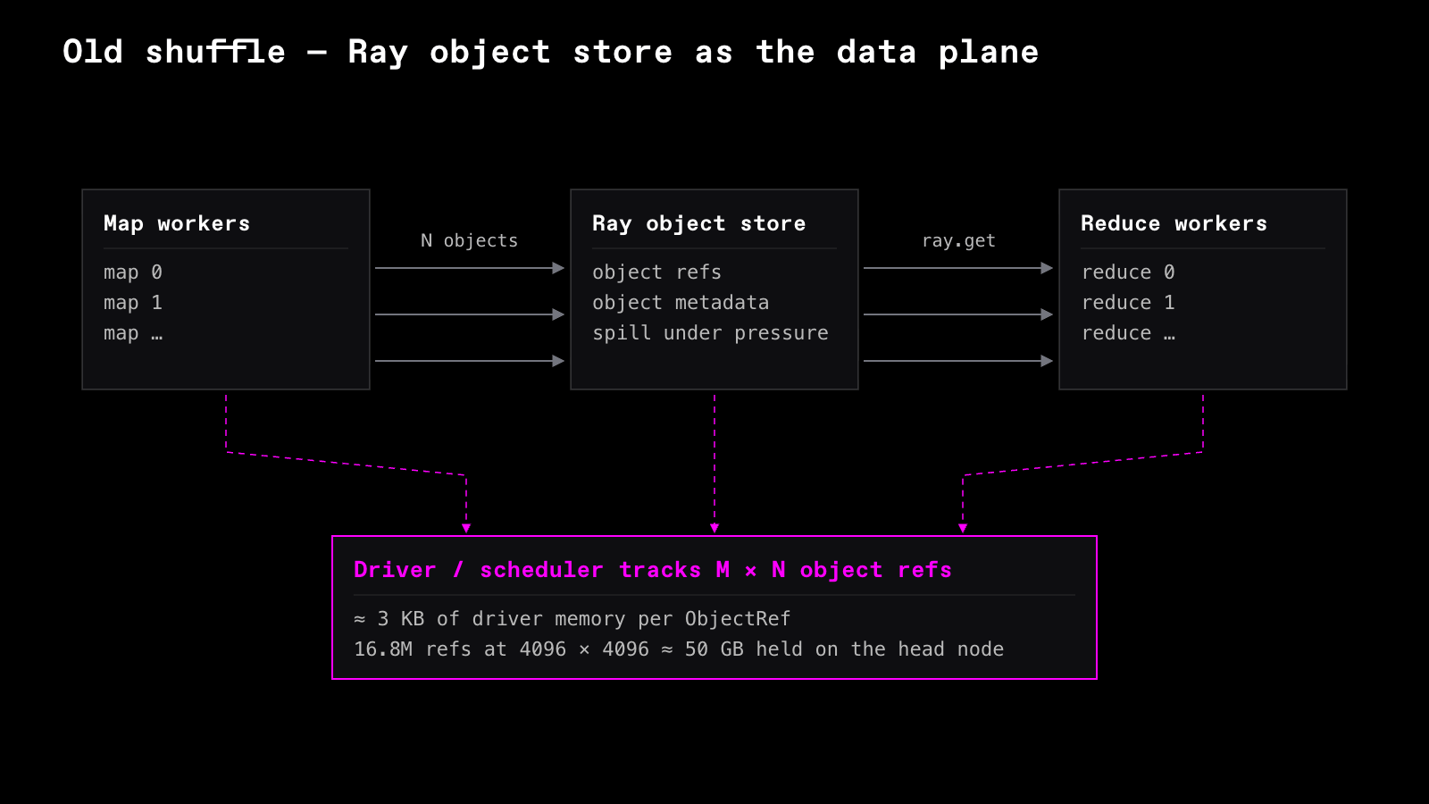
For moderate workloads, this worked well. The object store gives you locality-aware fetches, automatic spilling, and a clean programming model. Up to a few hundred gigabytes and modest partition counts, it was simple and effective.
The problem was the scaling model.
Three things broke down as partition counts grew:
1. The bookkeeping becomes the workload. Each of the M x N transfers became an ObjectRef, a handle the driver has to track and keep alive. By Ray's own accounting, each one costs about 3 KB of driver memory:
# ray/_private/ray_constants.py
# Each ObjectRef currently uses about 3KB of caller memory.
CALLER_MEMORY_USAGE_PER_OBJECT_REF = 3000
So driver memory grows linearly with the number of partition slots:
| Mappers x Reducers | Slots | Driver metadata |
|---|---|---|
| 1024 x 1024 | 1.05M | ~3 GB |
| 2048 x 2048 | 4.2M | ~12 GB |
| 4096 x 4096 | 16.8M | ~50 GB |
| 8192 x 8192 | 67M | ~200 GB |
Past a few thousand partitions, the driver spends its memory and CPU on shuffle metadata instead of coordinating the query. In our benchmarks this is exactly where the old shuffle begins to throttle:
- at 1 TB it exhausts head-node memory at 8192 partitions, and
- at 10 TB -- roughly 10x the map tasks, so 10x the references at the same partition count -- at just 1000 (see Benchmarking).
2. No control over spilling.
Shuffle data lives in the object store until memory pressure forces a spill. The store defaults to 30% of node memory, which comes out to ~19 GiB on our 64 GiB workers, while a 10 TB shuffle pushes ~310 GB through each of 32 workers. The object store is what decides when and what to spill primarily driven by memory pressure rather than by what the shuffle will read next. Additionally, the format and layout on disk are fixed, so Daft can't compress shuffle data on disk or lay it out for how the reduce side will read it back. As the benchmarks below show, compression alone is worth ~2.3x on bandwidth-constrained storage.
3. The reduce side can't stream.
A reduce task's arguments are materialized in full before its body runs, so the entire reduce partition (every mapper's contribution, concatenated) sits resident in memory before a downstream operator touches a single batch. The shuffle could not stream.
Put together, the limiting factor was no longer compute, network, or even disk bandwidth. It was the coordination and memory overhead of representing shuffle as millions of distributed in-memory objects.
We needed a different data plane.
Flight Shuffle: a disk-backed architecture
Flight Shuffle replaces the object-store-based shuffle path with a disk-backed, streaming data plane built around Arrow IPC and Arrow Flight.
The design comes down to a few core decisions:
- Disk is the data plane. Map tasks write shuffle output directly to local disk instead of materializing partitions in the object store.
- One file per mapper, not one file per partition. Each mapper writes a single combined shuffle file containing the data for every reduce partition.
- Arrow Flight serves shuffle data.
Every worker runs an Arrow Flight server that exposes shuffle partitions over
DoGet. - Everything streams. Shuffle data moves disk -> Flight -> executor as a continuous Arrow IPC stream without materializing whole partitions in memory.
- Metadata stays distributed. Reduce tasks only track lightweight logical partition references. Physical file layout and byte ranges remain local to the worker serving the data.
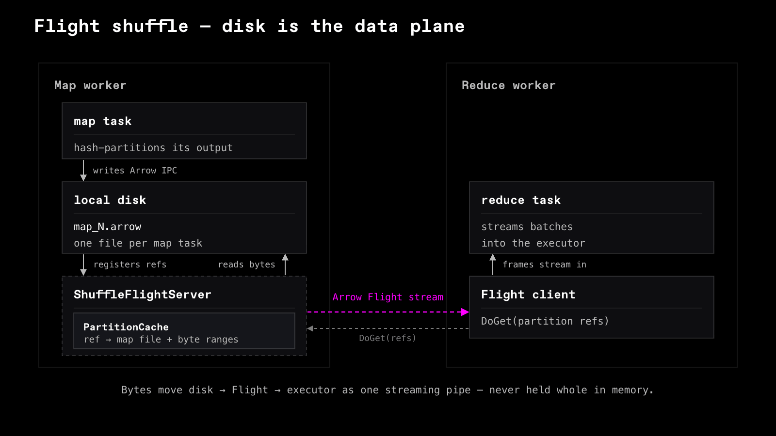
Together, these flip the three failure modes of the old design. Shuffle state no longer piles up on the driver: it stays local to the worker that wrote the data, tracked only as lightweight references. The bytes on disk are compressed Arrow IPC, designed for streaming reads. Reducers no longer wait on whole partitions: data streams disk -> Flight -> executor, so they start working before a partition has finished transferring.
The map side
Each map task writes its entire shuffle output into a single combined Arrow IPC file on local disk:
{shuffle_dir}/daft_shuffle/{shuffle_id}/map_{input_id}.arrow
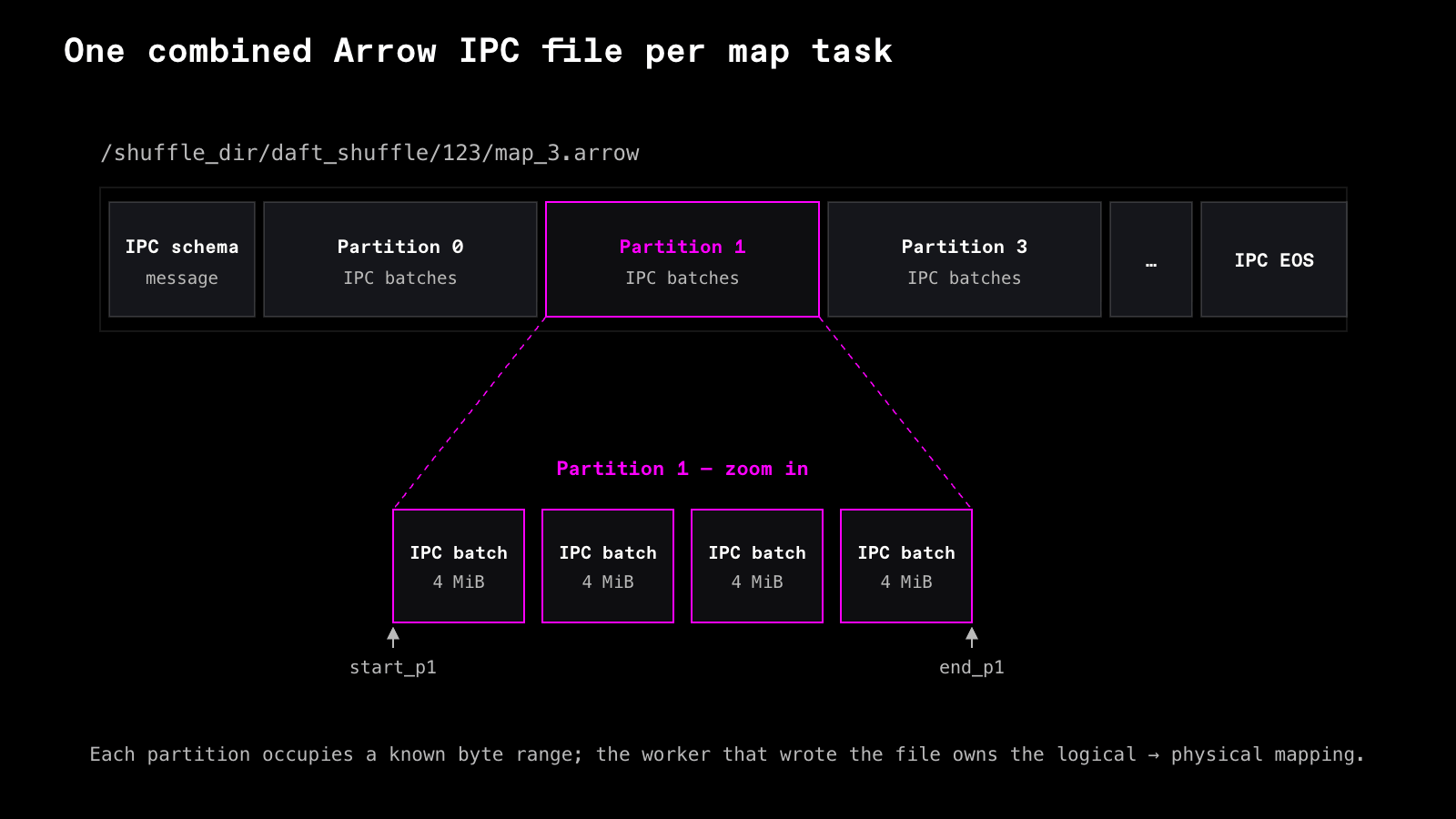
A single file per map task gives Flight Shuffle its map-side scaling and performance properties. The number of physical files stays proportional to the number of map tasks, not the number of map/partition pairs. The alternative of one file per map/partition pair does not scale. A shuffle with 4096 input files and 4096 output partitions would create over 16 million files. That many files would put pressure on file descriptors and inodes, driving millions of open/close syscalls, and leaving the scheduler with millions of tiny outputs to track.
Flight Shuffle separates the physical layout from the logical M x N shuffle matrix. Each mapper writes out one combined Arrow IPC file, each output partition occupies a known byte range inside that file, and the worker that wrote the file keeps the mapping from logical partition ID to physical location. Reducers and the control plane do not pass file paths or byte ranges around. They pass lightweight logical descriptors:
pub struct FlightPartitionRef {
    pub shuffle_id: u64,
    pub server_address: String,
    pub partition_ref_id: u64,
    pub num_rows: usize,
    pub size_bytes: usize,
}
When a reducer asks for a partition, the logical reference is resolved locally on the worker that wrote the data. That worker's ShuffleFlightServer maps the partition_ref_id back to the combined file and byte range for that partition.
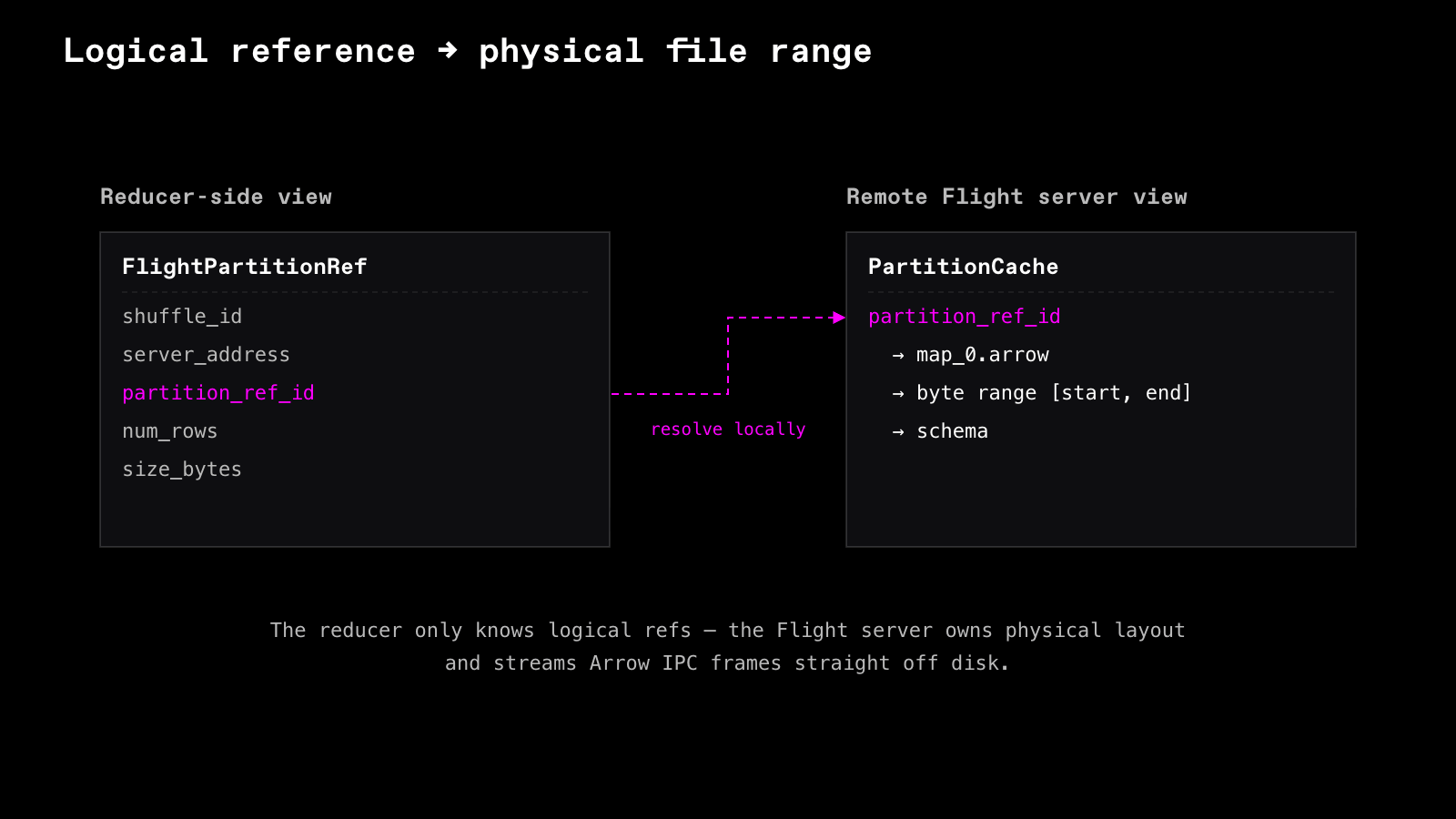
As a result, the only thing that moves between workers or sits in the control plane is the reference itself: a few integers and a server address. The shuffle's M x N matrix still exists logically, but not as M x N files or centrally tracked partition objects. File paths and byte ranges stay local to the worker that owns the data, keeping shuffle metadata small and distributed.
The rest of the map side is about writing that file efficiently. Three details matter:
- ~4 MiB IPC frames. Smaller frames add per-message and scheduler overhead; larger ones spike memory and delay the reducer, which can't touch a frame until all of it arrives. From our testing, 4 MiB balances streaming efficiency, pipelining latency, memory footprint, and gRPC framing overhead.
- Buffered, sequential writes. Frames go through a buffered writer, so they coalesce into large sequential disk writes instead of many small syscalls.
- Optional compression. The writer can compress frames with lz4 or zstd. Whether that helps depends on the balance between CPU, storage bandwidth, and network bandwidth (more on this in the operational guidance below).
A non-obvious bottleneck turned out to be task scheduling. Early versions spawned an async task per output partition. At thousands of partitions per mapper, the cost of spawning and polling those tasks started to rival the actual work of encoding each partition's record batches into Arrow IPC frames and writing them to disk. The fix was to write all partitions sequentially inside a single blocking task, which cut scheduler overhead and improved throughput at high partition counts.
The result is a map-side layout that preserves the logical M x N shuffle while storing it as one sequential, streamable Arrow IPC file per mapper.
The reduce side
Every worker runs an Arrow Flight server that serves the shuffle partitions sitting on its local disks. Reduce tasks fetch data with Flight's DoGet method, and request the logical partition reference.
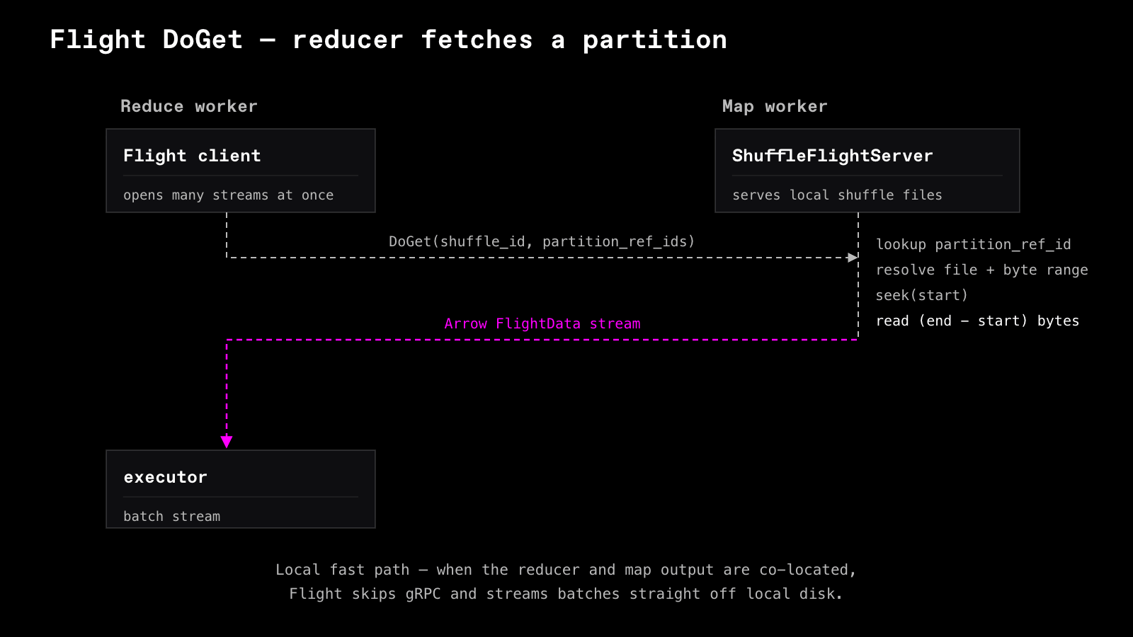
The server resolves the reference to a file and byte range, seeks to the offset, and streams the Arrow IPC frames straight off disk. It never reconstructs the partition in memory, and never decompresses or decodes a batch.
The payoff is on the consuming side. A reducer opens Flight streams to many map workers at once and forwards their IPC frames into the executor as they arrive. Under the old design, a reducer blocked until an entire partition had been reconstructed in memory, often gigabytes resident before a downstream operator saw a single batch.
The moment the first frame lands in Flight Shuffle, hash-table builders, aggregators, and sort partitioners start working while the rest of the partition is still in flight. Time-to-first-batch drops from "wait for the whole partition" to "wait for the first row".
Benchmarking
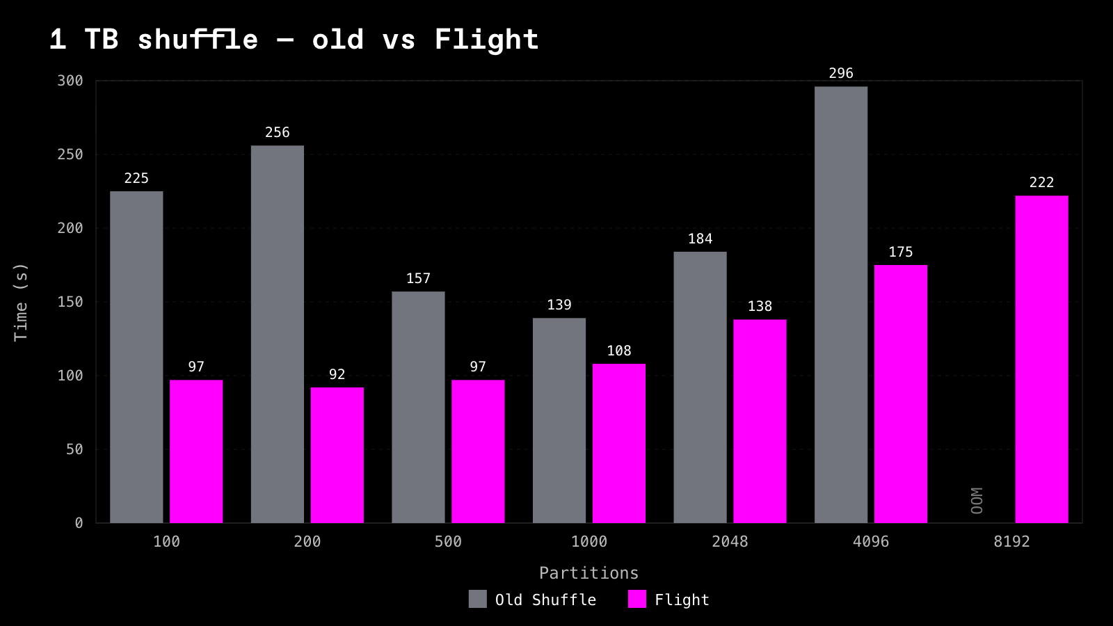
We benchmarked Flight Shuffle against our old shuffle using data from the TPCH dataset, at scale factor 1000 (~1 TB) and 10,000 (~10 TB).
Setup
- Datasets: TPC-H
lineitemat SF1000 (~1 TB) and SF10000 (~10 TB). - Operation: repartition
lineitembyl_orderkeyinto N partitions -- a pure shuffle, chosen to isolate the data plane from any join or aggregation compute. - Partition sweep: N in {100, 200, 500, 1000, 2048, 4096, 8192}.
- Cluster: 32 x AWS
i8g.2xlargeworkers (8 vCPU, 64 GiB RAM each),i8g.xlargehead node (4 vCPU, 32 GiB RAM). - Storage: 1875 GB local NVMe per worker.
Result: scaling with partition count
1 TB -- wall-clock seconds, lower is better:
10 TB -- wall-clock seconds:
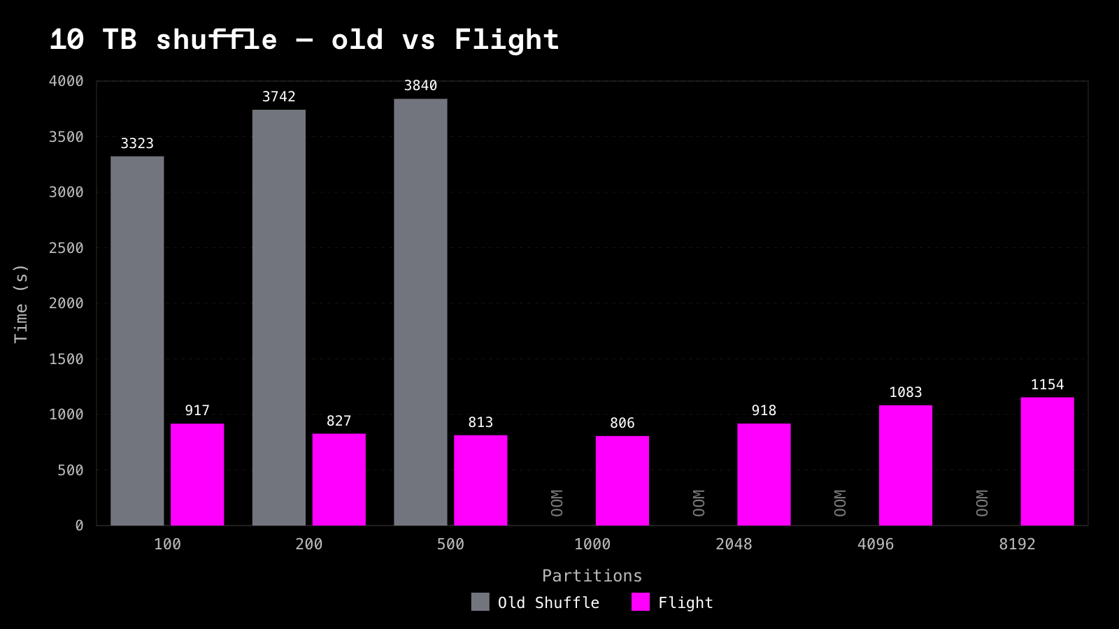
The failure point moves with data size, exactly as the metadata model predicts. At 1 TB the old shuffle survives until 8192 partitions; at 10 TB it OOMs from 1000 partitions on. Driver metadata scales with M x N, and 10x the data means roughly 10x the map tasks -- so the head node hits the same wall at a tenth the partition count. Flight Shuffle completes every cell in the sweep, because partition metadata never accumulates on the head node in the first place.
Where both complete, Flight is ~1.3-2.8x faster at 1 TB and ~3.6-4.7x faster at 10 TB. The gap widening with data size is consistent with the streaming model: the more a reduce partition outgrows memory, the more it costs to materialize it before downstream work can start, and the more it pays to never do that at all.
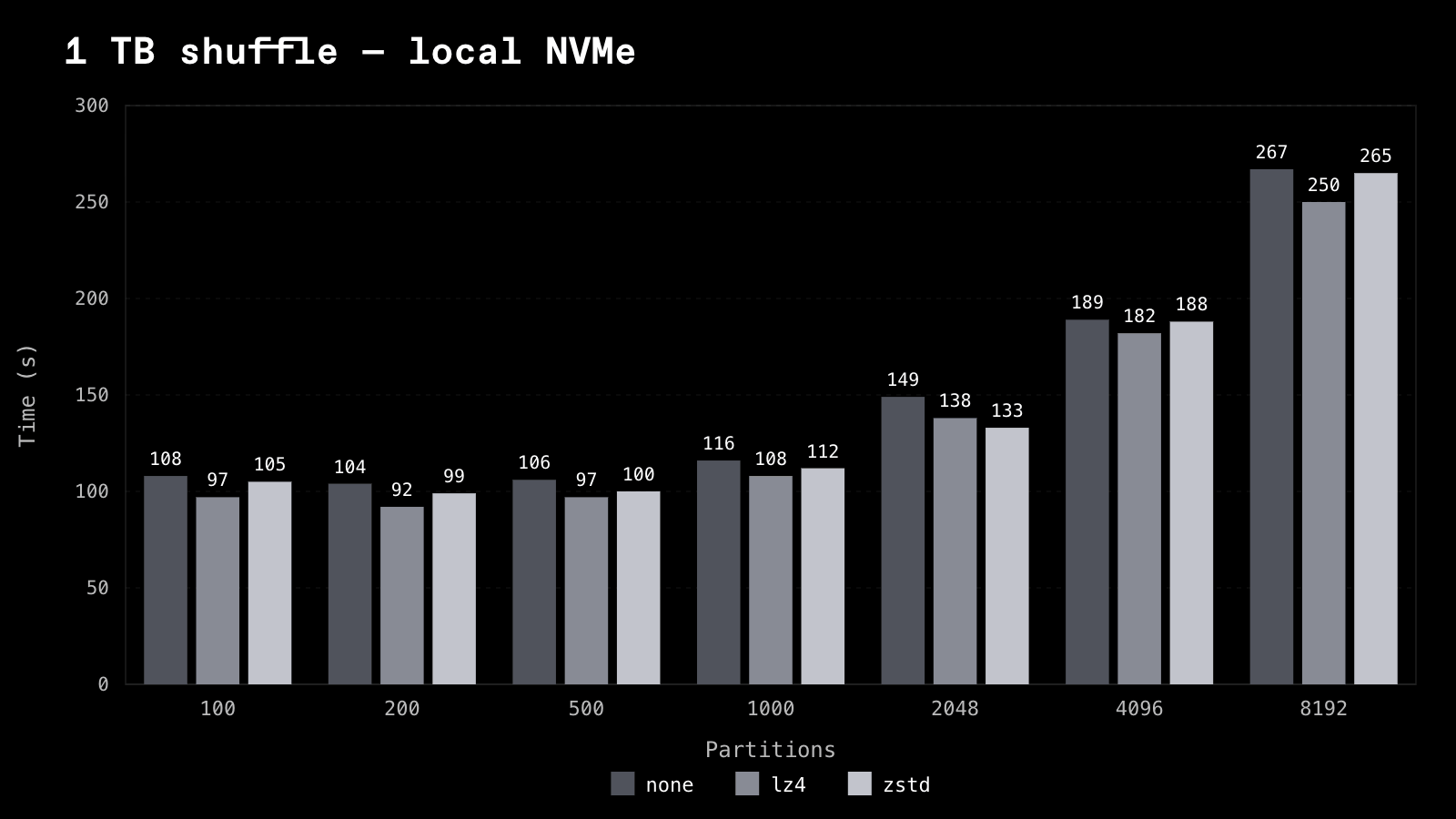
Compression
For Flight Shuffle only, we benchmarked the available compression codecs (None, lz4, and zstd) across disk types (EBS and NVME SSD). Compression trades CPU for bytes on disk and on the wire, so its payoff depends entirely on whether storage bandwidth is the bottleneck. The clearest way to see this is the same 1 TB shuffle on local NVMe versus network-backed EBS gp3.
For the EBS numbers, we used 32 x r8g.2xlarge workers, r8g.xlarge head node, 1875 GB EBS gp3 per worker.
1 TB, local NVMe -- wall-clock seconds:
1 TB, EBS gp3 -- wall-clock seconds:
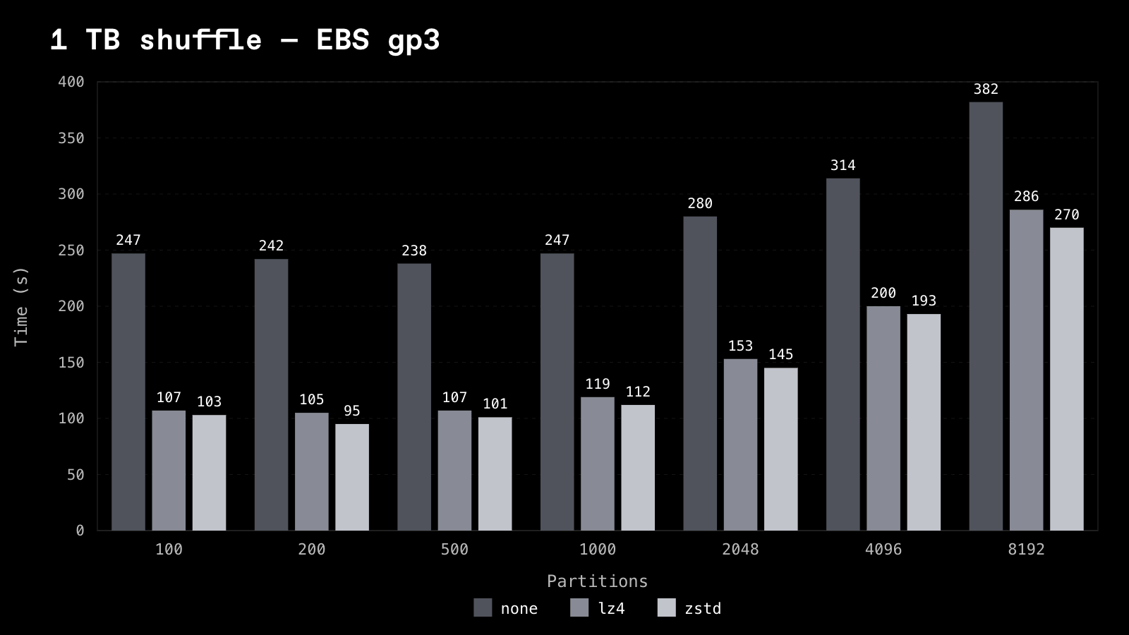
On fast local NVMe the disk isn't the ceiling, so lz4 buys a modest ~10%. On EBS, where storage bandwidth is the ceiling, lz4 is a ~2.3x win. An interesting insight is that lz4 is never slower than uncompressed, and it's dramatically faster when storage is constrained -- which is why it's the default. zstd compresses a little harder and edges out lz4 in every EBS cell -- by ~4-10% -- but costs more CPU and is a wash-to-slightly-worse on NVMe, so it's the pick when storage bandwidth is the known bottleneck rather than the default.
Operational guidance
Enabling Flight Shuffle
Flight Shuffle is enabled through Daft's execution config:
# /// script
# requires-python = ">=3.10,<3.14"
# dependencies = ["daft>=0.7.15"]
# ///
import daft

daft.context.set_execution_config(
    shuffle_algorithm="flight_shuffle",
    flight_shuffle_dirs=["/mnt/nvme0", "/mnt/nvme1"],
    flight_shuffle_compression=None,  # or "lz4" / "zstd"
)
Once enabled, repartitions, hash joins, distributed aggregations, and global sorts automatically use the Flight Shuffle data path.
Choosing shuffle directories
Every shuffled byte is written once on the map side and read once on the reduce side, so storage bandwidth sets the ceiling. Point flight_shuffle_dirs at the fastest local disks you have; if there are several, Flight Shuffle round-robins map output across them for aggregate throughput.
Compression
Compression trades CPU for bytes, and because the Flight server streams the mapper's bytes as-is, a frame is compressed once and stays compressed across disk writes, disk reads, and the wire -- decompression happens only at the reducer. So it pays off whenever storage or network bandwidth, not CPU, is the bottleneck. For flight_shuffle_compression:
lz4(the default) on fast local disk. Its CPU cost was low enough in our benchmarks that even on NVMe, where disk isn't the ceiling, it buys ~10%.zstdwhen bandwidth is the bottleneck. EBS or other network-backed storage, or clusters where cross-worker network is the constraint. When bytes are the limit, compression is the biggest knob available, and zstd's tighter ratio consistently beats lz4.Noneonly if you're CPU-bound on very fast storage. For example, several local NVMe drives whose aggregate bandwidth outruns what the CPU can compress through. Then compression spends your scarce resource to save a plentiful one.
Partition sizing
Daft picks partition counts automatically, but large workloads can benefit from tuning. Targeting ~128-512 MiB of post-shuffle data per partition balances scheduler overhead, reduce-side parallelism, memory, and skew tolerance.
Very high partition counts are now safe: Flight Shuffle removed the centralized metadata bottleneck that used to punish them. But larger partitions are still generally more efficient unless you specifically need high downstream parallelism.
Future work
Flight Shuffle has shipped, but a few directions remain open.
Adaptive compression
Compression is configured statically today, but the best choice depends on storage bandwidth, network throughput, CPU headroom, and how compressible the data is, all of which vary at runtime. A future version will choose between uncompressed IPC, lz4, and zstd dynamically, based on what it observes.
In-memory caching
Smaller shuffles that fit comfortably in cluster memory don't need to spill to disk. Even for larger shuffles, a partition is often fetched seconds after it was written. An in-memory layer on top of the disk backed IPC files could speed up our shuffles even more.
Disaggregated shuffle storage
Today each worker owns both query execution and shuffle storage. A separate shuffle tier can scale independently, open the door to elastic compute workers, longer-lived shuffle state, and shuffles larger than any single worker's local disk.
Conclusion
The object store modeled shuffle as millions of distributed objects for the driver to track, hold in memory, and spill under pressure. That model broke our shuffles at scale.
Flight Shuffle makes disk the data plane. Map tasks write Arrow IPC to local disk, Flight servers stream it across the cluster, and reducers process batches as they land. Shuffle metadata is lightweight, so the shuffle doesn't explode driver memory. The ceiling for shuffles has now moved to whatever your disks and network can sustain.
Flight Shuffle is available now. Turn it on with shuffle_algorithm="flight_shuffle". If you're running multi-terabyte joins, repartitions, or aggregations, we'd like to hear how it does on your workloads.
- Docs: https://docs.daft.ai/
- Source: https://github.com/Eventual-Inc/Daft

